Starting from the Ophidia VMI deployment (see Quick Start section), this section provides a simple Ophidia user session using the Ophidia terminal.
ll
to list the data cubes and containers in your session. Let’s consider PID_1 the identifier of your source data cube (for example http://127.0.0.1/ophidia/1/1).
oph_reduce2 dim=time;operation=avg;ncores=4;cube=<PID_1>
to reduce the whole data cube in a single value for grid point using the average along the time.
oph_explorecube
to visualize the first 100 values.
By default the Ophidia terminal will use the last output data cube PID.
So, apply:
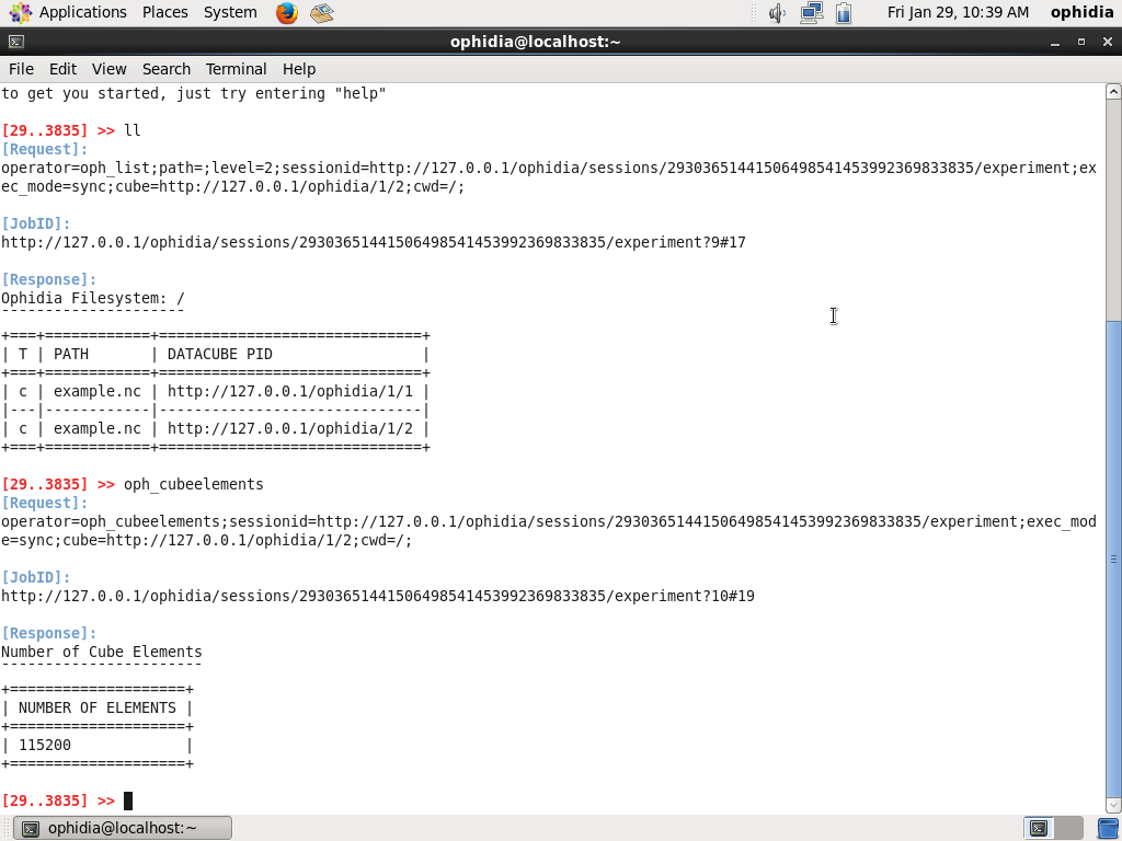
oph_cubeelements
to show the number of measured values
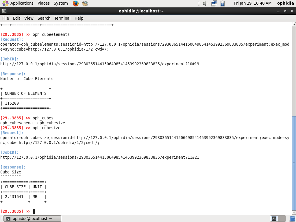
oph_cubesize
to show the size of your data cube
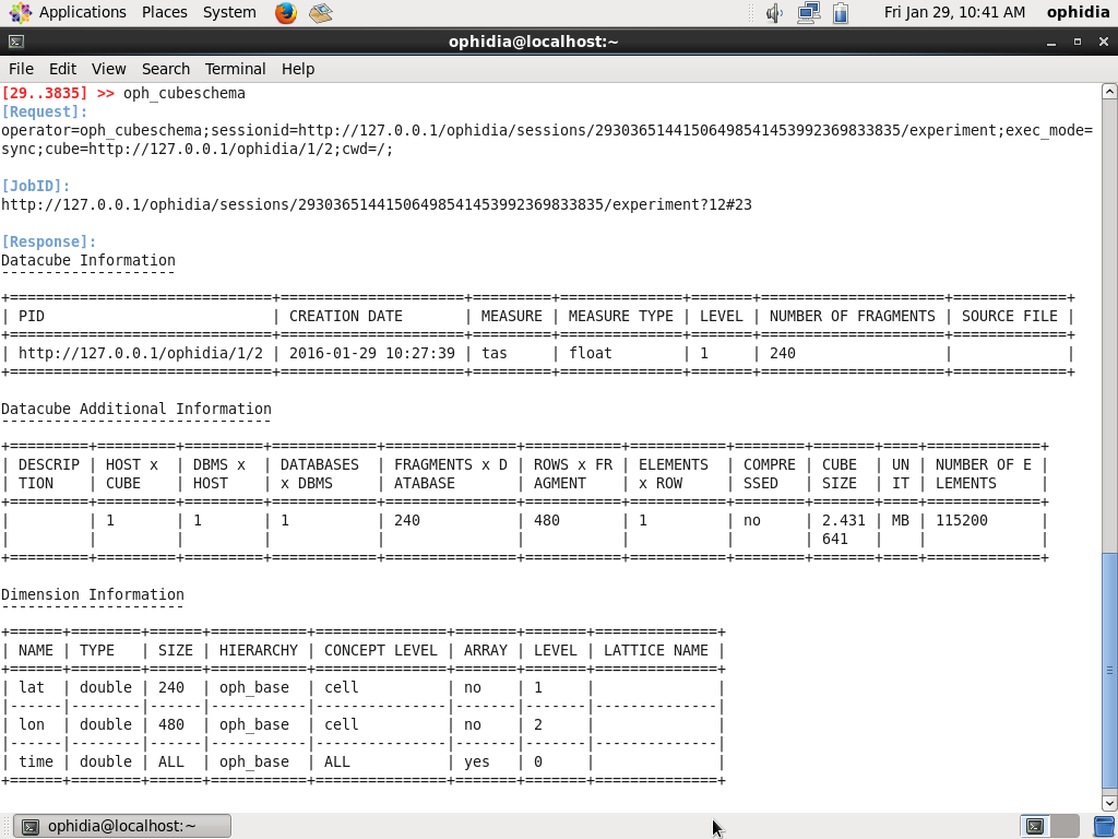
oph_cubeschema
to show information about the data cube, the dimensions related, the imported variable and types
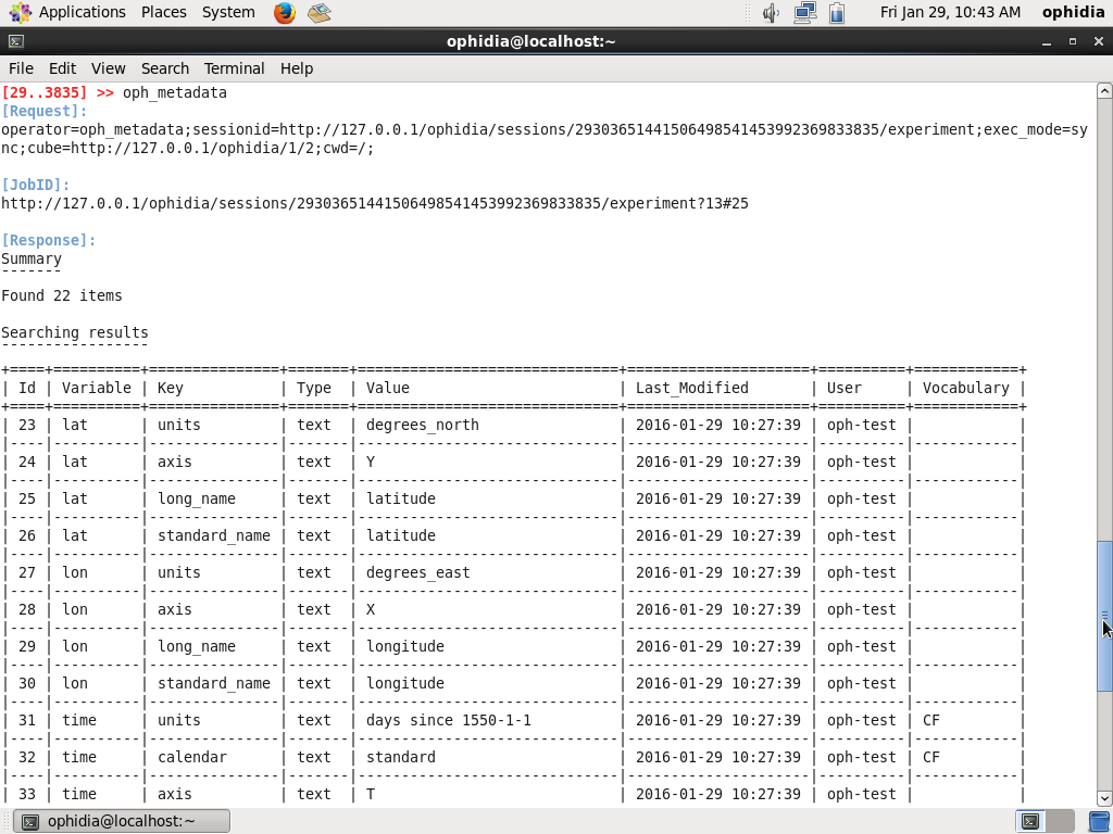
oph_metadata
to list the global and variable attributes
oph_subset cube=<PID_1>;subset_dims=lat|lon;subset_filter=27:81|-31:39;subset_type=coord;ncores=4;
to extract all the values related to Europe only from your source datacube
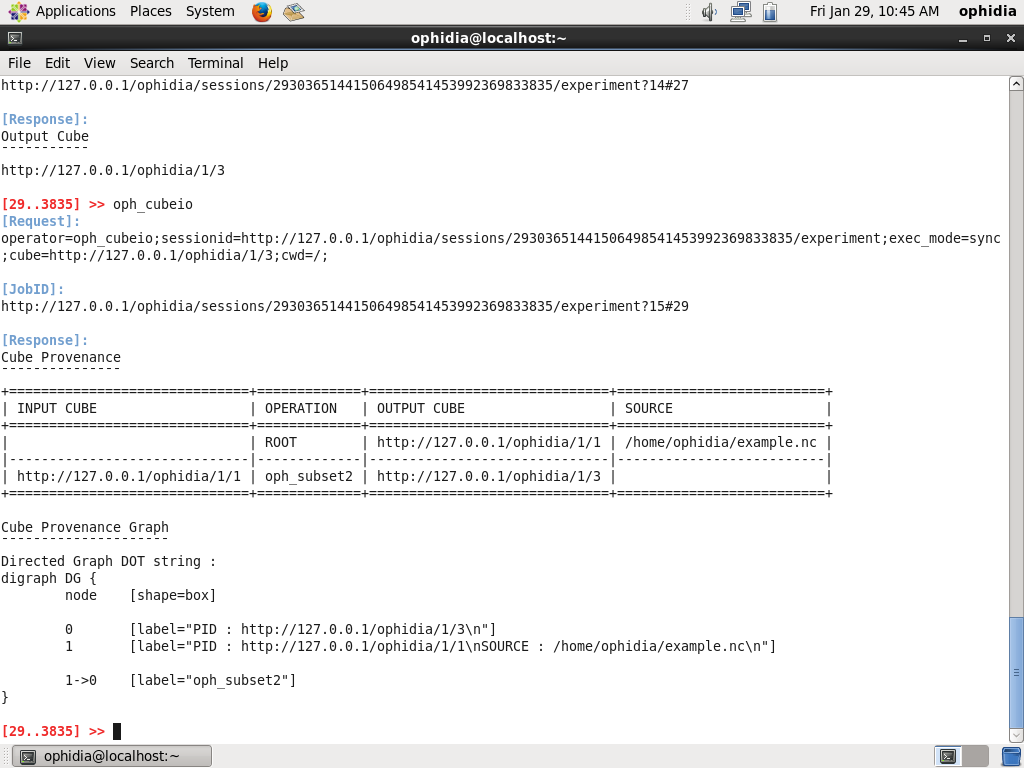
oph_cubeio
to show the data cube provenance
oph_exportnc2 output_path=<folder_path>;output_name=<filename>;ncores=4;
to export the data cube as NetCDF file; you can use “ncdump -h <folder_path>/<filename>.nc” to show the header
oph_apply cube=<PID_1>;query=oph_sum_scalar('OPH_<variable_type>','OPH_<variable_type>',measure,-273.15);ncores=4;
to convert from Kelvin to Celsius degrees.
OPH_<variable_type> represents the type of your data cube variable (e.g. OPH_FLOAT or OPH_DOUBLE). It is listed in the result of the oph_cubeschema operator
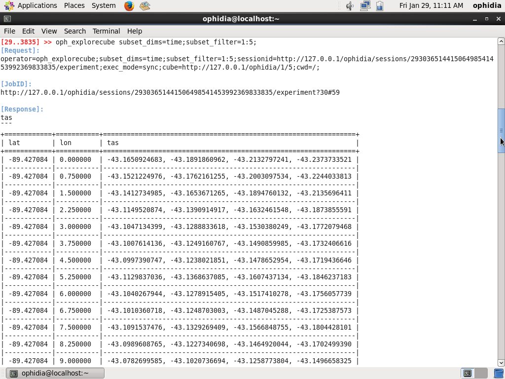
oph_explorecube subset_dims=time;subset_filter=1:5;
to show the results for the first 100 grid points and the first 5 time steps
oph_apply cube=<PID_1>;query=oph_gsl_boxplot('OPH_<variable_type>','OPH_<variable_type>',measure);ncores=4;
to extract the boxplot from the source data cube
oph_explorecube
to show the boxplot values for the first 100 grid points.